Conclusion

I've waited 2 weeks for your reactions and was happy to receive many, either by e-mail or as a comment here on this site.

This is a short summary of those reactions:
- systems are likely over-optimized and lack adaptability to different market conditions
- more criteria than just the Sharpe ratio are needed to select a system
- longer timeframes (e.g. 3-5 years) are needed to select a system
- subscriber should ask vendor if fundamental analysis is part of the system (not relying on only technical analysis)
- results cannot be generalized to all C2 systems, since analysis was limited to end-of-day stock systems
- recent market conditions were unusual

Here's my own opinion. First, I agree that out of the 100 systems I included, a substantial number could have been suffering from over-optimization. The problem is that it is hard to tell from the Sharpe ratio (and perhaps any other statistic) which system is likely over-optimized and which one isn't. I.e. if you have 100 over-optimized systems some of them will still show reasonable Sharpe ratios when going live (on C2) for a substantial amount of time.

Second, using more selection criteria than just the Sharpe ratio might be a good idea. However, these other criteria would need to have low correlation with the Sharpe ratio and still measure reward/risk in some way. Very difficult to find such criteria... An additional problem is that as we add more criteria we also increase the risk of over-optimizing the selection process.

Third, I agree that the longer the timeframe, the better. Ideally, it should include a period of severe Depression... Practically, we have to work with the data available and this is currently about 4 years, a period when the broader market gained a little less than 50%.

Fourth, having a good understanding of the system's underlying method might be a great selection criterion. The problem is, as a subscriber we can never reliably observe it. While the C2 stats are quite honest, we'll never know for sure about the vendor's underlying method as it depends entirely on what he says instead of on an independent third party's assessment.

Fifth, I also agree that results for future, options, forex, and intraday stock systems might look better or worse than what I showed here for end-of-day stock systems. I'll see if I can replicate the analysis for these other categories. A big problem here is that it is questionable if a subscriber could reproduce the hypothetical trades for some of the scalping system.

Finally, the recent credit crunch has done a lot of damage (not only to C2 systems, but to hedge funds as well). Remember though that the analysis includes many systems that were not affected by the credit crunch at all, e.g. in my first analysis (6 months, split into 2 periods of 3 months), only systems started in 2007 would be affected. But I'll see if I can redo the analysis without including data after May 2007.

One person also mentioned that some systems might have shut down while not closing positions. This could mean that results for the 2nd period look worse (or perhaps better...) than they really are, assuming a subscriber would have closed his positions once the vendor terminated the system. I understand this limitation, but as far as I can see it doesn't apply the majority of the systems in the tables I showed.

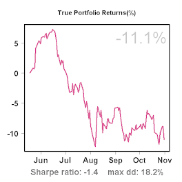
As I explained before these results were an important reason for me to suspend trading end-of-day C2 systems. Perhaps I will rerun the analyses a year from now when we'll have longer histories and see if things look more attractive then. To keep myself busy, I started a new C2 system myself: Kauai.

Some more analysis (3)

We're continuing the previous analysis, but instead of considering 3 and 6 months of history, we're now looking at 9 months:



The first thing we can see is that as the time periods get longer, the Sharpe ratios get smaller. Only one end-of-day stock system was ever launched on C2 with more than 18 months of history, and a Sharpe ratio > 2 for the first 9 months. I won't discuss all the details of the table, as by now I assume readers are familiar with interpreting these results (otherwise: see the previous 2 posts). However, what should be mentioned is the fact that 80% of the top-10 systems for the first 9 months underperformed the S&P 500 during the next 9 months, and in most cases by a substantial amount.

Extending the timeframe further, we get:



Before coming to a conclusion, I'd like to collect some feedback from readers. So what is your interpretation of all this?

Some more analysis (2)

In my previous post I compared the performance of the highest ranking systems during their first 3 months from inception to their performance during month 4-6. The conclusion of that analysis was that for all but one of the 10 highest ranking systems in the first period, performance during the 2nd period was substantially worse. Still, not taking into account transaction costs and slippage, the average Sharpe ratio of these 10 systems during the second period was slightly better than that of the S&P500 index.

Obviously the choice of 2 periods of 3 months each is arbitrary, and one could argue that 3 months is too short to judge the quality of a system. If that is true, we would expect to see more promising results if we would allow us a longer time period to evaluate a system before subscribing. So, let's look at the performance of 10 end-of-day stock systems with the highest Sharpe ratio's for their first 6 months:



As we can see, "Good NEWS Predictor" is again leading for the first period. However, this time performance during the 2nd period is quite disappointing. "Momentum #3" and "Momentum Breakout" show how bad it can get... We have to be a little cautious though, because I expect that at some point the vendor of Momentum #3 terminated trading the system without closing positions (while the equity curve continuous uncontrolled). In that case subscribers would have halted trading before digesting the full -0.68 Sharpe ratio. Momentum Breakout is quite a tragic case, as subscribers during the 2nd period found there account losing money during a runaway bull market (as indicated by the large negative excess Sharpe ratio).

Also of interest is Trend Plays #1. While it had a very decent Sharpe ratio (and equity curve) for the first period, in fact it underperformed the S&P500 index during that time on a risk-adjusted basis (as indicated by the -0.21 excess Sharpe ratio).

I didn't find these numbers particularly encouraging. Even with half a year of history it is quite a gamble what you'll get as a subscriber during the next 6 months for these systems that all had these attractive equity curves. In a way, it's interesting to look at some current end-of-day systems that will show up in this table half a year from now (i.e. they currently have about half of a year history).

Consider Small Cap Fundamental Value with a Sharpe ratio of 4.3 over 29 weeks:


It would show up right in between Momentun #3 and Good NEWS Predictor. Any guesses about its performance over the next 6 months??? I simply don't know. Perhaps it will do great, perhaps not. So far history suggests it's difficult to judge based on the Sharpe ratio.

Wave Rider (Sharpe ratio 2.2 over 27 weeks) is another system that will be included in the table 6 months from now:



We will continue with longer histories (9 and 12 months) in a few days.

Some more analysis

One of the reasons that led to my decision to terminate my portfolio was some analysis I did last week. It was motivated by my experiences in practice: in a few cases I had selected a system with great performance statistics, and it subsequently did quite well in my portfolio; but in other cases the performance was quite disappointing, even though at the time I signed up the system looked great.

So I decided to look at all end-of-day stock systems ever listed on C2 and see how often a "good-looking" system (based on the performance shown on C2) would continue to "look-good" in the future.

I further decided to define "looking-good" as: outperforming the S&P500 index based on the Sharpe ratio. With the underlying idea that I might as well put my money into the SPY (S&P 500 ETF) rather than going through all the trouble of trading if I have no reasonable expectation to get a better Sharpe ratio than the S&P500.

I only included systems with more than 10 trades, and started by taking all systems with a track record of more than half a year. Some of these started way back in 2004, others just 6 months ago; in other words they nicely spread out over time.

Next I downloaded the equity history for each system (using the C2 data api) and calculated the Sharpe ratio for the first 3 months after each system started, and then for months 4-6. What I would hope to see was that systems with a high Sharpe ratio in the first 3 months would also have a high Sharpe ratio in the next 3. Because when that is true, I could pick a system with a high Sharpe ratio as soon as it would have 3 months of track record and expect a nice result for the next 3 months when I would trade it myself!

It turns out, there are 75 end-of-day stock systems with more than 6 months of history. The table below shows the 10 systems with the highest Sharpe ratio for the first 3 months after they were launched:



The table shows that of all end-of-day stock systems ever launched on C2, no one had a Sharpe ratio higher than "Good NEWS Predictor" (4.22) for the first 3 months after inception. Trading it for the next 3 months would turn out to be a good choice, as it got an even higher Sharpe ratio (4.62) for that period. Interestingly, it did actually slightly worse during the first 3 months than the S&P500, as shown in the column Excess Sharpe ratio (i.e. the Sharpe ratio of the system minus the S&P500 Sharpe ratio over the same period). Unfortunately, the other 9 systems were less consistent, as they all did worse in the second period in terms of absolute Sharpe ratio and most did worse as well in terms of excess Sharpe ratio.

In fact--and this is where the trouble starts--half of the systems did worse than the S&P500 in the second period. On average they still outperformed the S&P500 Sharpe ratio by 0.51, but it's a difficult choice between getting the index return for sure, or having a 50/50 chance of out/underperforming the index.

The table also shows that when selecting one of these extremely well-performing systems for the first 3 months, there's a 3/10 chance of ending up with a loss in the next 3 months (negative Sharpe ratio).

As I am planning to show in a subsequent post, the 3 month period is actually a "best-case" scenario: The table looks much worse for many other periods (e.g. 4 months).

End of the Portfolio

As you've probably noticed, my portfolio has not been doing well for almost the entire past 5 months. Despite all my efforts to analyze systems, I have not been able to pick a profitable set of systems. Whereas the S&P500 is almost exactly back to where it was when I started my portfolio, I am sitting on a loss of 13% (excluding the P/L from my various put options to hedge, the loss would be even larger).

The main problems I have encountered can be summarized as follows:
- Technology issues with auto trading (extreme-os)
- Vendor decided to terminate/change system after major losses (Trend Plays #1, Longstoch-ST)

In addition, I was close to signing up for Positive Forex, which completely collapsed shortly thereafter.

Time to move on!

New hedge

The current put options on the Russell 2000 ETF (IWM) will expire in 2 weeks, so it's time to roll them forward. Therefore I sold (closed) the IWM Nov 72 puts today for $0.16 and bought (opened) the IWM Jan 72 puts for $1.26.

New Portfolio Weights

Starting this Monday, the optimal portfolio weights (for newly initiated positions) will change. Previous optimal weights were:
Weekend Trader: 32%
Trend Plays #1: 53%
ARS: 68%

Starting next week, the new weights will be:
Weekend Trader: 60%
Trend Plays #1: 49%
ARS: 41%

Since the weights sum to 150%, leverage will be about 1.5:1.

Nice (17%) Profit on WYY

Today, a limit was hit for a WYY position held by Trend Plays #1. Initiated on 6/4/2007, the trade yielded a nice 17% return.

Why are these distributions useful?

I ended my previous post with the words "Why is all this useful?", and today I'll try to answer this question.

Remember, I started discussing these distributions because Weekend Trader recently closed two trades with very large returns. Together with a trade with even larger returns (initiated in 2006) they have been responsible for almost half of the entire return (percentage-wise) of the system since its inception.

If you believe that these 3 trades are outliers, luck, the result of randomness etc, it would not make much sense to count on more of those for the future. After all, this is not about gambling but about trading. In that line of thinking, the performance of the system should be judged average at best.

However, if you believe these trades are an inherent part of the system's mechanics (perhaps due to a "let profits run" approach), the system (or vendor) should receive full credit for them, and performance might be judged good or even excellent.

The distributions we fitted can help to get more confidence in either the first ("luck") hypothesis or the second ("credibility") hypothesis, and allow us to determine how likely it is we can expect more of those big home-hitters in the future.

At first sight one might be tempted to conclude that since 3 out of 72 trades each resulted in increases on capital of more than 11%, the probability of this happening is 3/72 or 4.2%. I.e. we would expect every one out of 24 trades to increase equity by more than 11%. The problem with such an estimate is that it is not very precise: By the same calculation, the chance of observing a trade that increases equity by 10% (instead of 11%) is also 3/72, simply because none of the 72 trades so far showed a return between 10 and 11 percent. Similarly, the chance of observing a trade that increases equity with more than 12% (instead of 11%) falls quite abruptly to 1/72. Finally, if we would want to know the chance of a trade increasing equity by more than 17%, it would be zero, as we haven't seen those trades (yet)--but we all know that the chance is unlikely to be zero. Perhaps very small, but unlikely to be exactly zero.

Using distributions allow us to obtain more precise (and smoother) estimates. After fitting a distribution, we can get a precise estimate for whatever return percentage we are interested in, 10.4%, 10.8%, 200%, -30%, anything. It comes at a cost however: If we do a bad job at fitting a distribution, the probability estimate it will give us might be badly off. How badly? Consider the normal (Gaussian) distribution shown in red in the previous two graphs. Clearly it doesn't fit the histogram very well. According to this distribution, the chance of observing a trade that increases equity by more than 11% is only 0.27%! Compare this to the observed probability of 4.2%, and you see that this distribution underestimates the probability by a factor 15!

What do the other 3 fitted distributions have to say about the chance of observing a trade that increases equity by more than 11%?
- Cauchy: 3.7% (or 1 in 27 trades)
- Stable: 1.9% (or 1 in 53 trades)
- Generalized hyperbolic: 2% (or 1 in 48 trades)

These estimates look quite a bit more realistic than the Normal!

What about a trade that would increase equity by more than 20% (note: such a trade hasn't happened yet, so without fitting these distributions we wouldn't have a clue).
- Normal: 5.16e-08 (or 1 in 19,385,163 trades)
- Cauchy: 2% (or 1 in 51 trades)
- Stable: 0.7% (or 1 in 138 trades)
- Generalized hyperbolic: 0.5% (or 1 in 211 trades)

If we believe estimates from the last 3 distributions, such an event would not be that rare (the Normal estimate demonstrates once more how bad it is for fitting heavy-tailed distributions).

Based on these results, I have a hard time believing that these outlier trades are pure luck. I'm leaning more towards the second hypothesis: they're part of the characteristics of the system and should be treated as such. Obviously this doesn't mean it makes it a lot more comfortable to trade the system. It can be quite nerve-wracking to wait for the next big home-hitter... But analyses like these should give some confidence that it's worth waiting.

As you probably noticed, it can make quite a difference which distribution to choose... In subsequent posts I'll discuss how to measure and test how well a particular distribution fits the data, which might make such a choice a little easier.

Weekend Trader Alternative Distributions

As we saw last week, the normal (Gausssian) distribution doesn't fit the returns per trade of Weekend Trader really well. Therefore I fitted 3 alternative distributions that have been suggested for modeling of financial data:
- Cauchy
- Stable
- Generalized Hyperbolic

I will discuss some of their properties in subsequent posts. Let's first see what they look like:



The y-axis now shows the density (rather than the frequency, shown in the previous post). Not surprisingly, the 3 alternative distributions seem to follow the histogram much closer than the normal (red line) distribution. I obtained the parameters of all distributions through maximum-likelihood estimation (mle), an often used optimization method in statistics.

Why is all this useful, you might ask? Hang on, we'll discuss soon...

Weekend Trader Distribution of Trade Returns

Today, Weekend Trader closed two positions for a very nice return, both about 46%. Because the system always initiates trades with 25% of equity (4 open positions at any point in time), the two positions combined added 23% to the equity of the system.

Obviously the question is, how often can we expect to celebrate such nice trades? And, what is the chance of even larger profits? And, finally, what are the chances the system will close a trade for a 46% loss.

Over the coming weeks I will attempt to address these questions, by looking into the distribution of the trade returns of some systems, including Weekend Trader. To kick it off, let's look at a histogram of the Weekend Trader returns per trade.



The total number of trades since inception was 72 and most (29) of them yielded between zero and 2% on equity (i.e. between zero and 8% on the trade itself). The small bar at the far right represents a trade with a return of 16.7% on equity (66% on the trade itself) on a position in TFR held during the first half of 2006. The next bar (counting from the right) represents the two recently closed trades I described earlier.

The average of the return on equity (i.e. the expected return in statistics lingo) is 1.15% and the standard deviation is 3.54%. As a comparison, I plotted the normal distribution with this mean and standard deviation (red line). Visual inspection shows that the Weekend Trader returns are not normally distributed, as the peak is higher and the tails are heavier. This is confirmed by the 3rd and 4th moments of the distribution, i.e. the returns have a skewness of 1.85 and kurtosis of 5.29, while both are zero for the normal distribution.

Why is it important to note that the returns are not normally (Gaussian) distributed? Well, if they were, we could predict the probability and size of extreme returns quite easily. For example, we could predict that 95% of the returns fall within a range of ~2 standard deviations below and above the mean. However, if the returns are not normally distributed, such predictions can be misleading and (in this case) underestimate the chance of an extreme (positive or negative) return.

What I appreciate a lot in these returns, is that the extreme values all appear on the positive end of the distribution (and of course, I like extremely large returns). On the negative end, the bars of the histogram are all lying below the normal distribution, which is very good.

Rolling Correlations (3)

Earlier this week, I looked at 100-day rolling correlations between ARS and Weekend Trader, and between ARS and Trend Plays #1. This leaves one more combination for today: the correlation between Weekend Trader and Trend Plays #1:



This looks much more pleasant than the previous two graphs. For the most recent 100 trading days, the correlation between Weekend Trader and Trend Plays #1 is 0.26, which is only half of the correlation (0.52) between ARS and Trend Plays #1 for that same period. The max 100-day correlation between Weekend Trader and Trend Plays #1 is also quite reasonable: 0.37, substantially lower than the max 100-day correlation between Weekend Trader and ARS (0.62).

Rolling Correlations (2)

Yesterday, I looked at 100-day rolling correlations between ARS and Weekend Trader. Today, I'll show the same for ARS and Trend Plays #1:



The correlation between ARS and Trend Plays #1 for the last 100 trading days is higher (0.52) than the correlation between ARS and Weekend Trader (0.42). The upward trend that started about a year ago is still continuing.

Rolling Correlations

One of the reasons to trade a portfolio of systems (like I do), is to reduce volatility. This works best if correlations between the systems are as close to zero as possible. It is interesting to track rolling correlations over time, and the figure below shows 100-day rolling correlations between ARS and Weekend Trader (red line), and a 95% confidence interval (blue lines, based on a simple bootstrap with 1,000 replications). See this post for a more detailed explanation.



The figure shows that for the most recent 100 trading days, the correlation between ARS and Weekend Trader was 0.42, down from a recent high at 0.62. I consider these numbers quite high--I'd prefer to have systems correlate less, because otherwise it doesn't matter much (from a volatility perspective) if I would trade only one system rather than multiple systems. So, I'll keep monitoring and hope it'll come down a bit in the next months.

C2 Still Expanding

Six weeks ago was the last time I checked the number of newly added systems to the C2 universe of systems. It's time for an update:



During the last 30 days, 263 new systems were added. Not bad at all! The record of 365 new systems was set for the period 8/6 - 9/6.

Just for the five-day period from 8/29 - 9/2 as many as 166 new systems were added!
Of course, that is a little odd--so many systems in such a short period of time. So, I started to dig a little a deeper, and guess what? As much as 130 of these were from a single vendor. That must be quite a record. Even more peculiar: So far, none of these systems has made a single trade. Obviously, I'm very curious where this will go...

New Portfolio Weights

Starting this Monday, the optimal portfolio weights (for newly initiated positions) will change. Previous optimal weights were:
Weekend Trader: 9%
Trend Plays #1: 58%
ARS: 80%

Starting next week, the new weights will be:
Weekend Trader: 32%
Trend Plays #1: 53%
ARS: 68%

Since the weights sum to 153%, leverage will be about 1.5:1.

As a result of its good recent performance, statistics for Weekend Trader have improved substantially. Because it realized its recent gains in a time when ARS and Trend Plays #1 were mostly flat, it is not surprising that the portfolio optimizing algorithm was sensitive to this and let the weight increase substantially, from 9% to 32%.

"Vince Rowe Show" Interview

Here are the links to my interview on the "Vince Rowe Show" a few days ago. Each segment is about 10 minutes. We discuss C2, selecting systems, auto trading, slippage and many more things. Obviously 10 minutes is too short for a real in-depth discussion, but nonetheless I hope you'll enjoy it.

First segment

Second segment

Weekend Trader Surprise

As you might have noticed there haven't been that many posts during the last month. Part of the reason is that really not a lot happened to the systems in my portfolio. When I recalculated the weights two weeks ago, they were nearly identical to those I calculated in August. The portfolio P/L was oscillating a bit between -10% and -5%, and that was about it. However, last week I was pleasantly surprised by Weekend Trader soaring 25% to an all-time high.



The event confirms that sticking to a system is important. My experience so far is that profits usually come when you expect them the least.

Even though the system has a history of nearly two years on Collective2, the events of last week had a substantial impact on the statistics. For example, the graph below shows the Sharpe ratio and its BCa-bootstrapped (10,000 replications) 95%-confidence interval on each day, calculated using the data available up to the day of calculation (e.g. the left-most point of the curves is based on the first 100 trading days, the right-most point is based on the entire history of 486 trading days). The last five trading days caused the Sharpe ratio to jump from 0.82 to 1.31, which demonstrates how unstable these statistics can be--even with two years of data.



What we can learn from this is that there really is no point in preferring a system with a Sharpe ratio of 1.2 over one with a Sharpe ratio of 1, if they jump around all the time and have large overlapping confidence intervals. Most likely these differences are too small to be both statistically and practically meaningful. Instead of trying to pick the "best" system, we might be better off trading a larger number of "reasonably good" systems simultaneously.

Science Trader On Air!

Tomorrow (Thursday) between 12.15pm and 1pm EST, I will be interviewed by host Vince Rowe of the Online Trading Academy Dallas Radio Show. If you're interested you can follow the show by podcast or--if you're living in the Dallas area--on BizRadio 1360am.

New Portfolio Weights

Starting next week, the optimal portfolio weights (for newly initiated positions) will change slightly. Previous optimal weights were:
Weekend Trader: 13%
Trend Plays #1: 57%
ARS: 78%

Starting next week, the new weights will be:
Weekend Trader: 9%
Trend Plays #1: 58%
ARS: 80%

Since the weights sum to 147%, leverage will be about 1.5:1.

(Part of the reason not to leverage to 2:1, is that some equity needs to be available for the put options that I use to offset against the broader market)

Weekend Trader Backtest

A while ago, I asked the vendor of Weekend Trader if any backtest data were available. Initially, he send me several graphs. More recently however I received the underlying data, so I could do some more analysis. I think this can be very valuable because we can compare the backtest results with the hypothetical C2 results and see if there's any evidence of massive overoptimization in the backtest (note the emphasis of massive; I think a little overoptimization is unavoidable and not a problem).

The figure below shows the hypothetical equity curve starting on 10/26/1999, which is the beginning of the backtest. After 1,508 trading days, the curve is no longer based on the backtested returns, but instead on the hypothetical C2 returns (starting October 24, 2005); the border between these different periods is marked by the dotted line. I have scaled the equity to an index, starting at 100; and included the S&P500 returns over the same period, also indexed at 100. The y-axis has a log-scale, which means that if the daily return percentage would be constant, the equity curve would follow a straight line.



Visual inspection seems to suggest that until so far the C2 results don't deviate much from the backtest. In fact, the first 250 days of the C2 history look very similar to the last 250 days of the backtest period, in terms of the slope of the curve. I will compare some other aspects (drawdowns, alpha, beta, sharpe etc.) in subsequent posts.

Trend Plays #1 Did it Again

Again, a Trend Plays #1 trade was closed for a really nice profit today:

TCHC bought 6/22/07 for $11.13, sold today for $14.51 = 30% profit

The profit is actually even larger, because I bought some more on 7/2/07 for $10.77 as a result of a portfolio re-allocation.

(click to enlarge...)


Note the 45% drawdown early may--it's real, not a split!

What Happened to Positive Forex?

Six weeks ago, I opened a demo account with BulldogFX and subscribed to Positive Forex.

I was very happy with the demo, and pleased to see that the demo auto trade fills matched hypothetical C2 fills almost exactly. However, I was less pleased with the performance of the system itself:



Every now and then systems are blowing up spectacularly on C2, and I'm very worried that I found myself close to subscribing to the system. Because I didn't finish my analysis of the system, I don't know what my final decision would have been...

On a positive note, I have always been very suspicious of forex systems relative to stock systems, because I have seen many forex systems blow up before. That's one of the reasons why I've only traded stock systems in my portfolio so far. Perhaps if there have been a few systems on C2 with stable track records of more than 2 years, I might consider forex again, but in the near future, I'll stick to stocks.

A possible explanation why Positive Forex blew up is that it was generating high returns by ignoring hidden risk (i.e. a collapse of the carry trade). You can find a nice explanation here.

New hedge

Yesterday, Weekend Trader replaced three of its four positions. It has now reached the target weight of 0.13, as discussed here. Because leverage is lower now, I needed to readjust the hedge. I also found that hedging with the Russell 2000 index tracker ETF (IWM) gives a slightly better fit than hedging with SPY.
Therefore, I sold the SPY Dec 142 puts for $6 (bought last week for $8.30) and bought the IWM Nov 72 put for $2.33.

ARS Excess Sharpe Ratio

Please find below the 100-day excess Sharpe ratio for ARS. See here for an explanation of the excess Sharpe ratio.

(click to enlarge...)


As the figure shows, ARS outperformed the SPY on a risk-adjusted basis for most of the 100-day rolling windows, although recently it substantially underperformed. Testing for difference between the Sharpe ratio of ARS and the Sharpe ratio of the SPY over the entire history (590 trading days), we find that it's not statistically different from zero, as the 95% confidence interval is [-0.58, 1.81].

Excess Sharpe Ratio

A reader pointed out an interesting problem with rolling alphas that I showed two weeks ago: When the model fit is bad (as shown by a low R-squared), the interpretation of alpha and beta is not very meaningful. In such cases, alpha typically has a very wide confidence interval and tracking alpha over time is of limited value or even misleading.

So, if we're not really interested in the relation between a system and an index because we think such a relation is rather weak or non-existent, we could instead compare the Sharpe ratio of the system to the Sharpe ratio of the index.

The figure below (upper panel) shows the 100-day rolling Sharpe ratio for Trend Plays #1 and the S&P 500. The difference between the two Sharpe ratios, which I call the system's excess Sharpe ratio, is shown in the lower panel. Most of the time the excess Sharpe ratio of Trend Plays #1 is greater than zero, i.e. the 100-day rolling Sharpe ratio of Trend Plays #1 is greater than the 100-day rolling Sharpe ratio of the S&P 500 index. In other words: The system does better than the index on a risk-adjusted basis.



The bad news is that the difference is not significantly different from zero (with 95% confidence) for any of the 100-day periods shown in the plot. Even when we construct a confidence interval for the difference between the Sharpe ratio of the system and the Sharpe ratio of the S&P using all 294 trading days, the difference is not significant: A bootstrapped confidence interval for the difference (with 10,000 replications, bias-corrected) shows [-0.886, 3.039].

Hedge Roll-over

I just changed the SPY put option hedge from the Dec 144 to the Dec 142 contract. This keeps the option delta such that the portfolio is approximately market-neutral. The Dec 144 contracts were purchased for $4.80 on July 31 and sold for $9.20 today. The Dec 142 contracts were bought for $8.30.

C2 still expanding

About six weeks ago, I posted a graph that showed the number of new systems launched on C2 for the past 30 days. The updated figure (as of today), looks like this:



It seems the current market volatility doesn't reduce the enthusiasm to launch new trading systems on C2. In fact, the number of newly launched systems (~220) has never been as high as last month.

Approximate Entropy

Many traders and investors prefer an equity curve as smooth as possible. It gives a sense of predictability, i.e. in our minds we extend the curve in the future and the smoother it is, the more confident we feel about our prediction. In many cases the Sharpe ratio is capable of summarizing the smoothness of the curve in a simple number, and the higher its absolute value, the smoother the curve.

Now, think about the Sharpe ratio of a sine wave for a moment...

Even though it's zero, we would be extremely happy to find a trading system with an equity curve represented by an exact sine wave. We would simply get into any open positions at the bottom of the wave and get out at the top, and repeat this over and over again for a huge profit.

Although this is an extreme example, it nicely shows that we might not only be interested in the smoothness of an equity curve, but also in the amount of randomness. I.e. it is possible that two systems have the same Sharpe ratios, while one system is less random than the other due to some much more subtle patterns not captured by the mean or standard deviation.

An interesting measure to quantify "randomness" in financial time series was published in the Proceedings of the National Academy of Sciences by Pincus and Kalman(*) about 3 years ago, based on a mathematical approach and formula called Approximate Entropy introduced in the early nineties by Pincus.

I won't go into all the details of this measure except for noting that it is rooted in the concept of information entropy developed by Shannon in 1948 as part of information theory (Wikipedia is a good first start for those who want to investigate further). Outside the world of finance, it has also found its application in the medical world (e.g. irregularity of heart rate). Approximate Entropy (ApEn) is a number, and the higher it is the more irregular (random) a time series. Thus, when applying ApEn to the daily returns of a C2 system, we would prefer a lower number over a higher number. ApEn requires 2 parameters: a block or run length (usually 1 or 2) and tolerance window (usually 20% of the standard deviation). In all figures below I use a block length of 1 and 20% of the standard deviation as tolerance windows, denoted as ApEn(1, 20% SD). The daily log-returns are used as inputs.

Over the entire history of a system, I got the following figures for the systems in my portfolio:
Trend Plays #1: 1.74
Weekend Trader: 1.95
ARS: 1.77

We can also do a rolling ApEn, estimated over 100 trading days:



This figure suggests that the equity curve of Trend Plays #1 has become more irregular (random) over time.



For Weekend Trader no such trend exists. Note that around the 400th trading day, ApEn was at its lowest point, suggesting relatively high regularity. This is reflected in the steady pattern of peaks and troughs in the equity curve during the preceding 100 trading days.



Finally, for ARS, we see yet a different curve. ApEn increased gradually over the past year, somewhat similar to what happened for Trend Plays #1.

These numbers and figures don't give an immediate clue how to improve returns and they also seem to be quite close across the systems. Pincus and Kalman show an example where a strong increase in ApEn preceded the Nov 1997 crash in the Hang Seng Index (HSI). I'll look for a C2 system that crashed and see if I can relate the crash to the system's ApEn in a future blog post.

(*) Pincus S, Kalman R E. Irregularity, volatility, risk, and financial market time series. Proceedings of the National Academy of Sciences 2004; 101(38): 13709-13714.

A few Words about the Drawdown

As you must have noticed, the portfolio drawdown gets larger on an almost daily basis, i.e. 17.8% from the peak, 11.8% from the day I started this blog, and 8.9% since I made a major change in the portfolio on July 23 (terminating auto trading and extreme-os, and including Longstoch-ST and ARS).

So, let's analyze what's going on:

1. About half of the 17.8% drawdown from the previous peak is due to a drawdown before the major portfolio change, and about half is due to a drawdown after that date. In other words, I experienced two consecutive drawdowns on 2 different portfolios.

2. All systems in the new portfolio, except Trend Plays #1, are setting fresh max drawdowns every day:
ARS -9.71%
Weekend Trader -15%
Longstoch-ST -13.44%
Note, however that these started earlier than July 23. Losses since July 23 are about 8% per system on average.

3. Because I was leveraged, these losses were bigger in my portfolio. At the same time I was partly hedged (only fully hedged beyond S&P500 drawdowns of ~7%), so ending up with a portfolio drawdown of 8.9% since July 23 is nothing unusual.

4. The next few days will be interesting. If the sell-off continues, I will become fully (delta) hedged (because the SPY Dec 144 puts will start to have delta's < -0.5) and I will start to roll these over to lower strikes (to avoid becoming over-hedged). On the other hand, if the market rallies we have to hope that the systems will keep outperforming the market (i.e. their returns should exceed the losses on the puts).

5. Experiencing this drawdown has many positive sides. First, we can see the systems perform during adverse market conditions. This will only benefit me, as it allows a more robust selection of systems in the future. Second, I have learned that it will probably pay off to spend some time on improving the hedge, e.g. estimate betas with more advanced models, backtest various hedging strategies and use of multiple indices.

Longstoch-ST confusion

Apparently my previous post on Longstoch-ST caused some confusion. It was not clear whether I was forced to close my positions because the system will be terminated by the vendor or whether this was my own decision. To clarify: I decided myself to close the open positions this morning at the open, while I could also have decided to keep them open and wait for the official signal from the vendor to close the positions, possibly at a later date.

I understand that the vendor is planning to blend Longstoch-ST signals with signals from one of his other systems on C2, and launch this as a new system.

New Portfolio Weights

The weights of the current portfolio positions (excl. Longstoch-ST) are as follows:
Weekend Trader: 55%
Trend Plays #1: 73%
ARS: 14%

The new optimal weights will be:
Weekend Trader: 13%
Trend Plays #1: 57%
ARS: 78%

This sums up to 148%, which means leverage will be about 1.5:1

It might take a while before the actual positions will reflect these weights as Weekend Trader and Trend Plays #1 can hold positions for several weeks.

Longstoch-ST termination

I just got a note from the vendor of Longstoch-ST that he is considering terminating the system in its current form due to the recent drawdown. This means I have decided to close any open positions tomorrow at the open and delete the system from my portfolio.

On the one hand it is very unfortunate that I had to digest the full drawdown because it just started after the first signal I received. On the other hand its effect could have been much worse if this was the only system I was trading, or if I did not have my positions hedged.

I think I should have taken the downward trend in its alpha much more seriously, as that has actually been a greater concern to me than the current drawdown (which seems to follow the sell-off in the broader market closely).

You might remember I had to terminate extreme-os during a drawdown last month because of technical problems. I think I solved that problem successfully by sticking to end-of-day systems (terminating auto trading). I now have to terminate another system during a drawdown because the vendor decided to change the course/terminate it. This is something that will be much harder to prevent in the future. In fact, it is likely that many systems will be terminated once a heavy drawdown occurs, as subscribers are probably all fleeing away and new subscribers will be hard to attract with a major drawdown on the record.

On the other hand, the declining alpha (see yesterday's post) should have given a clue that something was not ok, and I regret that I didn't do this analysis before I subscribed.

Longstoch-ST alpha and beta

We continue with rolling alpha and betas, and examine results for Longstoch-ST:



Similar to what we noticed for Weekend Trader yesterday, alpha shows a steady decline from 0.18% per day over the first 100 trading days, to -0.10% for the most recent 100 days. Contrary to Weekend Trader, beta has not been increasing but was fairly stable, fluctuating between 0.46 and 0.81.

A test for a linear trend in alpha showed that alpha has been declining with 0.00133 percentage point per day, which is quite a bit steeper than Weekend Trader. The decline is almost significantly different from zero at the 90% confidence level (p = 0.119).

Weekend Trader Rolling Alpha and Beta

This post will be similar to the recent one on Trend Plays #1, but with results shown for Weekend Trader:



Things don't move in the right direction for Weekend Trader currently, which is unfortunate. Alpha shows a slow but steady decline from 0.12% per day for the first 100 trading days to -0.04% for the most recent 100 trading days. At the same time beta has seen a steady increase from 0.38 to 0.87. Or, in other words, for the last 100 trading days, the system pretty much had the same volatility as the S&P500 with no excess returns. I don't know the reason behind these trends, but I would like to see them reverse (i.e. increasing alpha and decreasing beta). The fact that my portfolio optimizer started to give smaller weight to Weekend Trader in the portfolio is consistent with these results, and when the trend would reverse I'd expect to see the optimal portfolio weight for Weekend Trader go up again.

I checked whether the trend was statistically significant (using the same model as discussed for Trend Plays #1), but it wasn't. (tau = -0.00044% per day, with standard error of 0.%, which means it's not statistically different from zero at both the 95% and 90% level).

A possible explanation for the declining alpha could be that as more people started to trade the system over time, the increase in order size started to affect the entries and exits of the system. Therefore, I estimated the rolling alphas and betas again, assuming that all transactions did not take place on Monday at the open (which is the official entry/exit point the vendor uses), but instead on Monday at the close:



As we can see, no clear difference. Hence we can rule out that explanation.

Hedge roll-over

I just rolled-over the SPY put option hedge from the Sep 144 to the Dec 144 contract. The September contracts were purchased for $1.55 on June 1 and sold for $2.80. The Dec 144 contracts were bought for $4.80.

Trend Plays #1 Rolling Alpha and Beta

During the past week I have discussed alpha, beta and R-squared for Longstoch-ST and ARS. These statistics are essential in understanding how much better or worse the system did in comparison to some index (e.g. the S&P 500).

I estimated these statistics for a single point in time, using the entire history of the system available at that (most recent) date. However, it is quite possible that alpha and beta vary over time and that will be the topic of the next few posts.

I calculate rolling alpha's, beta's and R-squared in order to track their change over time. I started with the first 100 trading days and calculated the stats. Then I re-estimated everything using day 2-101, then day 3-102 etc. all the way till the last day of the available history. This is a similar approach to the rolling correlations I estimated a few weeks ago.



The graph in the upper-left corner shows rolling 100-day Alpha's for Trend Plays #1 have varied between 0.05% and 0.35%, i.e. the system outperformed the S&P 500 by at least 0.05% per day on average for any 100-day period since its inception. The statistic is always represented by the red line, the blue lines mark the 95% confidence interval. The graph in the upper-right corner (rolling beta) shows that in the beginning the system was a lot more volatile than the index, probably because it used more than 1x leverage at the time. We can see that since it stuck to 1x leverage more recently, beta has always been smaller than 1 for any 100-day period.

The lower-left corner graph shows that R-squared has been fairly low--it fluctuated between 0.15 and 0.30. Again, a low R-squared is desirable in general, but makes alpha and beta harder to interpret. Finally, I have included the 100-day return for the S&P500 in the bottom-right corner. The reason for this is that we always need to judge alpha and beta in light of the movement of the index. For example, normally we don't like zero alpha, but if a system would only show zero alpha during a strong bull market, combined with a high beta for that period, it simply means the system took advantage of the bull market at the right time. This is what seems to have happened with Trend Plays #1 since day 200: Alpha steadily declined, while S&P500 returns increased--which shouldn't be reason for panic in light of the explanation above.

Obviously an interesting question is whether alpha is declining over time. Looking at the graph it seems to fluctuate, but without a clear trend. We can test this formally by extending the standard regression with a linear time trend, i.e. the model is:

R = alpha + beta * I + tau * days,

where R is the system's daily return, I the S&P500 index daily return and days the number of trading days since the start (this is applied to all the data, not just 100 days). If we estimate the parameters of the model (alpha, beta and tau) through linear regression, it turns out that tau equals -0.0008% and alpha 0.30% per day. With such a decline the model would predict an alpha of zero or lower after day 375 (0.3 / 0.0008), which is less than hundred days from now! Fortunately, the standard error for tau is extremely large (0.001%) relative to tau itself, and hence the effect is far from significant. So, it's not something to be worried about currently, but I will keep a close eye on it in the coming months.

ARS Alpha and Beta

Alpha and beta for ARS look pretty good:

(S&P 500)


(Best fitting index)


These figures represent alpha and beta for ARS, their 95% confidence intervals, and the fit of the model (R-squared) using daily, weekly and monthly returns. In the uper panel, the S&P500 index is used as a benchmark. In the lower panel I picked the best fitting benchmark (based on R-squared statistic).

We can see that ~30% of the movement of ARS can be explained my the movement of the various indices (an exception is the model for monthly returns where the S&P500 index explains only 21%--here it pays off to pick the S&P100 instead).

The excess returns over the S&P 500 (alpha) are 0.058% per day, 0.30% per week and 1.27% per month, with all betas smaller than 1. Again, as with Longstoch-ST: excess return and lower volatility than the benchmark are good. Note though that the R-squared is higher than with Longstoch-ST, i.e. this system seems to follow the broader market a bit closer.

For those interested, these are the graphs:

ARS Sharpe Ratio

Last week I discussed the Sharpe ratio of Longstoch-ST, and today I'll follow up with the same analysis for ARS:

Sharpe ratio = 1.49
95% CI [0.18 , 2.68]

To get an idea about these numbers we can compare them to the SPY (S&P 500 ETF), which could have been an alternative option for the same period of 574 trading days:

Sharpe ratio = 0.83
95% CI [-0.46, 2.12]

and we can see that the Sharpe ratio for ARS is almost twice the Sharpe ratio for the SPY (buy & hold).

As before, it is of interest to watch the Sharpe ratio converge as the number of observations gets larger:



The figure shows the value of the Sharpe ratio at each point in time (using the history available at that point), starting when the system is 100 days old (red line). I also shows the confidence interval, which is estimated with the bootstrap method (10,000 replications), using the percentile method (purple) and the preferred BCa (Bias-corrected and accelerated, green).

It seems as if the most recent 200 observations have not changed the estimates of both the Sharpe and its confidence interval much, so the estimate of 1.49 looks pretty stable to me, and not likely to change very sudden.

As before, we can check if any autocorrelation issues exist by plotting some lags:



Contrary to Longstoch-ST, there's actually some autocorrelation present at lag 7 and 17, exceeding the 95% confidence bounds. This is an issue that requires further investigation because autocorrelation can possibly affect both the Sharpe ratio and its confidence interval. I'm curious if the effect will be substantial (I don't think so, but you never know) and I'll come back to this after the weekend.

Alpha / Beta Plots

For those who prefer a visual representation of the information in my previous post, have a look at the plots below:



The plot in the upper-right corner shows for each day (dot) the system's return (vertical axis) and the index' return (horizontal axis). The red line is the linear (least squares) regression line, with slope equal to beta and intersection with the horizontal axis equal to alpha.

The plot in the lower-left corner shows the same for weekly returns, and the plot in the lower-right corner shows monthly returns. Finally the plot in the upper left corner shows equity curves and indices using daily data (colors correspond to colors used in daily, weekly and monthly plots, e.g. green = Nasdaq Bank etc.)

Longstoch-ST Alpha and Beta

An important question when deciding on including a system is whether it merely tracks an index (possibly leveraged), or whether it is capable of showing good performance irrespective of what the broader market does.

This question can be answered by examining alpha and beta, which are two coefficients obtained after regressing a system's returns on an index' returns. I estimated alpha and beta for Longstoch-ST, their 95% confidence intervals, and the fit of the model (R-squared) using daily, weekly and monthly returns. The index is the S&P500 and results are shown below:



The first thing to notice is that the model fit is extremely poor, as the R-squared is only 0.13 (using daily returns), which means that only 13% of the movement of Longstoch-ST can be explained my the movement of the S&P500. This is good news! The lower the R-squared the better, as I like to deal with vendors capable of picking winning trades without just taking advantage of the index (which, as we all know, did quite well over the last year). The only disadvantage of a low R-squared is that interpreting the alpha and beta coefficients becomes less meaningful.

Still, they look the way we want them to look: positive alpha and beta < 1. Using weekly returns, alpha is 0.59, meaning the system generated an average return of 0.59% per week in excess of any S&P500 return. Ideally, alpha would be statistically different from zero, indicated by a lower bound of the 95% confidence interval greater than zero. We can see that alpha is statistically different from zero for both weekly and monthly returns but not for daily returns. Beta is 0.64 for daily returns, meaning that when the S&P500 index was up (down) 1%, Longstoch-ST was up (down) 0.64% on average. In other words: the system generated returns in excess of the S&P500, with less volatility than this index. That's the best you can get!

Also of interest is the negative sign for monthly betas. It suggests that on a monthly basis the system would be up when the index would be down. However, the number of observations (N) is only 11 and the fit of the model poor, so it doesn't mean anything at this point.

Of course, we don't have to restrict ourselves to the S&P500 index. I repeated the same exercise for 36 other indices (shown at the bottom of this post), and picked the ones with the best fit (highest R-squared):



It apparently pays off to examine other indices as well, because the fit (R-squared) has improved a lot for both weekly and monthly data. Apparently the Nasdaq Bank index is a better matching index than the S&P500 at the weekly level. However, I consider these figures still very low: Out of the 37 indices considered, none was able to explain more than 25% of the variance of the system's returns. With better fitting indices we basically see the same pattern for alpha (positive) and beta (smaller than one). All in all, these statistics played a major role in picking this system and I hope the system will continue to show low R-squared, small beta and (most important) positive alpha.

The indices I included were:

DOW JONES COMPOSITE INDEX
DOW JONES INDUSTRIAL AVERAGE IN
DOW JONES TRANSPORTATION AVERAG
DOW JONES UTILITIES INDEX
NYSE COMPOSITE INDEX
NYSE International 100
NYSE TMT
NYSE US 100
NYSE World Leaders
NASDAQ BANK
NASDAQ BIOTECHNOLOGY (DRM)
NASDAQ COMPOSITE
NASDAQ COMPUTER
NASDAQ FINANCIAL 100
NASDAQ INDUSTRIAL
NASDAQ INSURANCE
NASDAQ NNM COMPOSITE
NASDAQ OTHER FINANCE
NASDAQ TELECOMMUNICATIONS
NASDAQ TRANSPORTATION
NASDAQ-100 (DRM)
S&P 100 INDEX
S&P 400 MIDCAP INDEX
S&P COMPOSITE 1500 INDEX
S&P SMALLCAP 600 INDEX
AMEX COMPOSITE INDEX
AMEX INTERACTIVE WEEK INTERNET
AMEX NETWORKING INDEX
DJ WILSHIRE 5000 TOT
MAJOR MARKET INDEX
NYSE Arca Tech 100 Index
PHLX SEMICONDUCTOR SECTOR INDEX
PHLX THESTREET.COM INTERNET SEC
RUSSELL 1000 INDEX
RUSSELL 2000 INDEX
RUSSELL 3000 INDEX

VGZ (Trend Plays #1) closed for +11.6%

VGZ, a trade from Trend Plays #1, was closed today for a nice 11.6% profit:
entry 6/22/2007 $4.58
exit today $5.11

(click to enlarge)

New Portfolio Weights

As I discussed in other posts this month, I have terminated extreme-os and decided on trading Longstoch-ST instead. Another (4th) system I will include is ARS, which has a history of over 2 years on C2. I will discuss the reasons for including both systems in subsequent posts this week, and for now will stick to the new portfolio weights:

Weekend Trader: 20%
ARS: 65%
Trend Plays #1: 56%
Longstoch-ST: 59%

(note that as before the weights sum up to 200% to reflect 2:1 leverage)

The current weights of Weekend Trader (48%) and Trend Plays #1 (72%) in my account are somewhat different from their new weights. To transition to the new weights, I could sell part of shares for each position. However, these systems hold positions quite long and I may find myself adjusting positions every month, which becomes quite costly in terms of commissions and spreads. Therefore I have decided to change the weights more gradually, i.e. whenever a new trade will be issued for Weekend Trader and Trend Plays #1 this new position will be scaled using the new weight and hence it might take a few weeks/months before the system settles on its new weight (i.e. when all positions have been renewed).

This also means that currently, I can't allocate the full 65% and 59% to ARS and Longstoch-ST (unless I would accept more than 2:1 leverage) and instead will settle for 40% for each. From now on I will post the real weights regularly and monitor how they converge to the target weights.

Longstoch-ST Max Drawdown per Trade

Yesterday I posted some results on the average return per trade, and in this post I'll look at the average risk (in terms of drawdown) per trade. The figure below shows for each of the Longstoch-ST trades the maximum drawdown of the trade. E.g. if a position was opened for $100, closed for $110, and moved all the way down to a low of $95 in between, the max drawdown of that trade would be 5%.



Looking at the figure, we can see that most trades had a max drawdown between 0 and 6%, while three were a lot larger than the rest (-18%, -13% and -17%). Similar to calculating the expectancy (average return), we can calculate the average max drawdown by taking the average of the length of the bars in the figure, which happens to be -2.73%. We can use the bootstrap to estimate a confidence interval:
95% Percentile [-3.60 , -2.00] ; BCa [-3.79 , -2.10]
99% Percentile [-3.93 , -1.82] ; BCa [-4.21 , -1.94]
(100,000 replications)

These ranges are quite acceptable for me, in particular when taking into account that the drawdown as a percentage of equity is half of these numbers (because the system enters each position with 50% of equity).

The only things that are a little worrying are the few exceptionally large drawdowns. And here we can see the benefits of trading a portfolio of systems! Suppose the weight of this system in my portfolio would be 40%, in that case an 18% per trade drawdown would equal to a 3.6% drawdown on equity (18 x 0.5 x 0.4), which I think is large but still manageable nonetheless.

The vendor actually suggests subscribers to consider a stop-loss between 12 and 25% (the latter being the stop-loss imposed by the vendor), but I'll stick to just following the signals as they are issued by the vendor to match the system's C2 track record as closely as possible.

Longstoch-ST Per-Trade Statistics

In my previous post on Longstoch-ST I used the daily returns as the unit of observation. In this post I'll switch to the individual trade as the unit of observation. Longstoch-ST has made 70 trades so far, and the graph below shows the percentage P/L (return) per trade (i.e. a position opened for $100, and sold for $110, would show up as 10%). The trades are ordered by the date they were entered. Because the system enters each position with exactly 50% of equity, the account P/L percentage resulting from each trade is half of the P/L per trade.



Two things you'll probably notice immediately is that most of the trades were closed with a profit of 2%, and that there were two trades with large losses (relative to the other trades). Also, more of the recent trades resulted in a loss compared to the older ones.

Despite these losses, the system has a positive expectancy (average return per trade) of 1.17%. I estimated bootstrap confidence intervals at the 95% and 99% level, using both the percentile and BCa method (100,000 replications):

95% Percentile [0.32 , 1.92] ; BCa [0.18 , 1.83]
99% Percentile [0.03 , 2.13] ; BCa [-0.21, 2.00]

Note the large difference between the (simple) Percentile and (advanced) BCa method for the lower bound at the 99% level (0.03 vs -0.21, positive vs negative expectancy).

To get an idea how this first outlier return (-16.9%) affects these results, let's repeat without this trade included:

mean return = 1.44%
95% Percentile [0.80 , 2.05] ; BCa [0.77 , 2.02]
99% Percentile [0.59 , 2.24] ; BCa [0.55 , 2.20]

I think the results including the first trade were pretty good, but this looks even better. The question is: What was going on with this first trade, how likely is it that we'll see this happening in the future, and with what frequency?

It turns out this particular trade was NTAP, entered 7/11/2006 31.41, closed 7/17/2006 26.11. From the chart (below) we can see that the trade was not the result from a sudden overnight gap due to some unexpected earnings news etc. It was bought in a short-term downtrend, which unfortunately did not reverse. As such I put more value on the first set of estimates (including the trade). Because it happened only once so far, there's very little we can say about how often it is expected to occur again.



Tomorrow I'll post some results on drawdowns per trade and discuss how a stop-loss (as the vendor suggests to his subscribers) would have worked out.

Nice Profit on Trend Plays #1 Trade

It has been a while ago since the last trade closed for Trend Plays #1 in Mid-June. This morning a limit was hit on CACS, however, and it was closed for a very nice (+29%) profit.

Thank you!

I started this blog exactly two months ago, and since then there have been 1,400 unique visitors and over 3,200 page views. I'm very motivated to continue this effort and hope it will benefit many. Feel free to post any suggestions how to further improve this blog, as I'm always open to change.

First Positive Forex Auto Trade Demo Results

Two weeks ago, I started trading Positive Forex in a BulldogFX demo account, using C2's "2nd generation autotrading".

The first couple of trades were closed yesterday, and the fills match the C2 hypothetical fills very well.

These are the trades shown by C2:



And this is what I got in my demo account:



Obviously the entry fills do not match, because these trades were already open before I started the demo. For the EUR/AUD position the exit fill in my demo account was 3 pips better than the hypothetical C2 fill. For the other two positions, AUD/USD and USD/CAD the fills were identical. Also note that the scaling worked nicely: the 70 minilots for EUR/AUD and USD/CAD appeared in my demo account as 1 minilot, while the 140 minilot AUD/USD appeared as 2 minilots.

another extreme-os missed signal

I just missed another (exit) signal for extreme-os (SYNL). This turned what is shown by C2 as a winning trade into a losing trade in my account. I have decided to terminate autotrading immediately to protect my trading capital.

extreme-os missed trade

Yesterday I missed an extreme-os trade, GDP, that closed today for a substantial profit. It was missed due a technical problem, and we're still figuring out what the cause of the problem was. It seems my decision to terminate auto trading on my PC was right. The extreme-os subscription ends at the end of this week, and I will announce the new portfolio weights (including Longstoch-ST) very soon.

Longstoch-ST Sharpe ratio

The first thing I usually look for in a system is a high Sharpe ratio. It is reported, together with its confidence interval by C2:

Sharpe ratio = 2.2
95% CI [0.14 , 4.2]

To get an idea about these numbers we can compare them to the SPY (S&P 500 ETF), which could have been an alternative option for the same period:

Sharpe ratio = 1.5
95% CI [-0.6, 3.6]

The system does quite a bit better, I'd say!

Now, these are all estimates for a single point in time (today). Last month's estimate was likely different, and so will next month's estimate be. But as more observations (days) become available, we might expect these ratios to converge and the confidence interval to narrow. I like to watch this convergence over time, and hence I plot the value of the Sharpe ratio at each point in time, starting when the system is 100 days old (red line). I also plot the confidence interval, which I estimate with the bootstrap method (10,000 replications), using the percentile method (purple) and BCa (Bias-corrected and accelerated, green). I won't go into detail about the difference between the green and purple line, except for noting that the BCa (green) method is usually considered a superior estimate.



What we can see from the graph is that the Sharpe ratio was declining steadily from about 3 around day 100 to about 2 around day 200, and seems to have settled around 2 between days 200 and 250. Meanwhile the lower bound of the 95% confidence interval has been fluctuating between -0.5 and +0.5 with no clear trend.

All in all, I don't see any alarming patterns, and in an ideal scenario the Sharpe ratio would converge around 2 over time with the confidence interval narrowing further. This would also be close to the 5-year backtested results (2.14 Sharpe ratio) posted by the vendor on C2. I would consider a Sharpe ratio of 2 as quite good, and few end-of-day systems available on C2 show considerably higher Sharpe ratio over a similar or longer period.

One concern about using these bootstrap methods for confidence intervals is that they may be unreliable in case returns are autocorrelated. So to be sure, we check for autocorrelation, by plotting the correlation of the return at day t with the return at day (t-1), (t-2), ..., (t-12) and see if any of these lags are correlated. Results are shown below, and suggest that none of these correlations are significant (i.e. the bars stay within the horizontal bounds), which means that we can safely use these bootstrap methods for the Sharpe ratio confidence intervals.

How long until you're a millionaire?

The vendor of Trend Plays #1 brought to my attention the existence of a handy free calculator to calculate the final equity with compounded returns:

calculator

I like these tools a lot, as they nicely demonstrate the incredible power of compounding. For example, an annual return as low (or high, whatever you prefer to call it) as 30% will turn $100K into $10MM within just 16 years.

If you want to get rich and have time, all you need is a steady annual return around 20-40%.